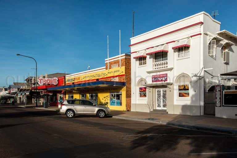
Inelastic demand and a monopoly supply.
Prices for water, fresh fruit and vegetable costs more in Outback Australia than in capital cities, this can be linked to the limited supply (usually only one supermarket) (aka a monopoly) and relatively inelastic demand by consumers.
ACARA Alignment: ACHEK017
Clip Length: 0:24 minutes
Year: 2026
URL: https://youtube.com/shorts/2pConRlc5GM?si=kBzw39028rldpWP4
Economics Concepts: Supply, opportunity cost, inelastic demand, monopoly
- Bring in something students can’t easily get in the school canteen – for example Uber Eats deliver a fast-food meal to the classroom
- As students enter the classroom hand them a random amount of fake money (e.g. Monopoly money)
- Invite students to bid on how much they will pay for the food using their Monopoly money. Give the item to the highest bidder.
- Enquire why students think the price went above what it would be if it was purchased at the store (you might have to steer them towards a limited supply in the schoolroom market)
- Now show students the Outback YouTube clip above
- Ask students to identify what type of market it is (oligopoly, monopolisitc competition, perfect competition or a monopoly). Students should be able to identify that is is a monopoly market.
- Following the clip ask students about the similarities with the monopoly money food auction and the Outback. Hopefully they will see that a limited supply, higher opportunity costs of shopping elsewhere and relatively inelastic demand for necessities like bottled water means prices are higher than in urban centres.
- Next display a map of the school and local area and locate the nearest supermarket. Then set the location to Bedourie, Queensland. Identify that the nearest supermarket for Bedourie residents is in Boulia or Birdsville either a 195 or 187km trip down the road!
- Now draw an inelastic demand curve, such as the one below and show how even if the supermarkets in the Outback increased the prices for water and fresh produce there would be a limited decrease in demand
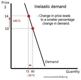
- Use the diagram to complete the following question:
If Broccoli costs $10 per kg in Longreach and 80 kg are sold in November. What is the price elasticity of demand if the price increases to $14 per kg and 72 kg are sold in the first week in December?
Write equation: P.E.D = % change in Price / % change in quantity
Calculate separately the % change in quantity
(Q2-Q1) / ((Q1+Q2) / 2)
= (72-80) / (80+72)/2)
= -8 / 76 = -0.1052
Calculate separately the % change in price
(P2-P1) / ((P1+P2) / 2)
= ($14-$10 / ($10+$14)/2)
= $4 / $12 = 0.3333
Put it together:
Price Elasticity of Demand = % change in quantity / % change in price
= -0.1052 / 0.3333 = -0.3158
Evaluate the outcome: A $4 (or 33.33%) increase in price will decrease the quantity purchased by 10.52% and has a PED of -0.3158, which is less than 1, so demand for broccoli in Longreach is inelastic. - To conclude the lesson and cement their knowledge, get students to play this Wayground quiz https://wayground.com/join?gc=55625753